Code 401 Class 05 Reading Notes

Linked Lists

What are Terms(found in terminology section of the above link)

1. A data structure that contains nodes/points to the next node in the list.
2. This refers to the number of references a node has. It also is means that there is only one reference, and the reference points to the Next node in a linked list.
3. This refers to there being two references within the node. It also means there is a reference to both the Next and Previous node.
4. These are the individual items/links that live ina linked list. Each of these contain the data for each link.
5. Each node contains a property called this term. This property contains the reference to the next node.
6. This is a reference of type Node to the first node in a linked list.
7. This is a reference type Node to the node that is currently being looked at. When traversing, you create a new one of these variables at the Head to guarantee you are starting from the beginning of the linked list.

---

Big O: Analysis of Algorithm Efficiency

Big O(oh)

notation is used to describe the efficiency of an algorithm or function. This efficiency is evaluated based on 2 factors:

1. Running Time (also known as time efficiency / complexity) The amount of time a function needs to complete.
2. Memory Space (also known as space efficiency / complexity) The amount of memory resources a function uses to store data and instructions.

Overview

Big O’s role in algorithm efficiency is to describe the worst case of efficiency an algorithm can have in performing it’s job.

Consider the 4 key Areas for analysis:

1. Input Size
2. Units of Measurement
3. Orders of Growth
4. Best Case, Worst Case,and Average Case

Input Size

Refers to the size of the parameter values that are read by the algorithm.This does not only take in the number of parameters the reads, but the size of each parameter value as well.

Units of Measurement

Quantifying Running Time, Three Measurements of time are considered

1. milliseconds from the start of a function execution until it ends.
2. Number of operations that are executed
   • Think of this as the number of lines of code that are executed from start to finish of a function.
3. The number of **“Basic Operations” that are executed.
   • “Basic Operation” refers to the operation that is contributing the most to the total running time. This is typically the most time consuming operation within the inner most loop.

Quantifying Memory Space, *Four sources of Memory Usage are considered

1. The amount of space needed to hold the code for the algorithm
   • Think of this as the number of bytes required to store the characters for the instructions specified in your function.
2. The amount of space needed to hold the input data.
   • If direct input data is not considered, we may just refer to this as Additional Memory Space since not all functions have direct input values.
3. The amount of space needed for the output data.
4. The amount of space needed to hold working space during the calculations
   • Working Space can be thought of as the creation of variables and reference points as our function performs calculations. This will also include Stack Space of recursive function calls … specifically how memory usage scales relatively with the size of the input.

Orders of Growth

As the value of n grows, the Order of Growth represents the increase in Running Time or Memory space.

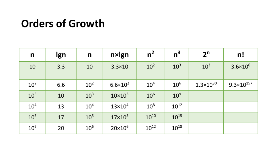
Complexity factor compared to input size n.

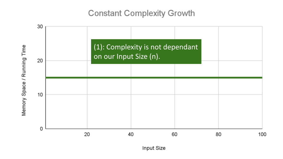
Constant Complexity means that no matter what inputs are thrown at our algorithm, it always uses the same amount of time or space.

The below algorithm as an O(1) constant efficiency, no matter the size of a or b, this function simply returns the sum of those 2 numbers.

ALGORITHM Sum(number a, number b)

   number val <-- a + b
   return val

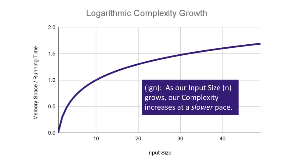
Logarithmic Complexity represents a function that sees a decrease in the rate of complexity growth, the greater our value of n.

The following algorithm loops through an array and creates a sum of their values. It has to perform a set number of operations for every value that our input of size n holds.

ALGORITHM SumArray(arr[0...n - 1])

    number sum <-- 0

    for number i <-- 0 to n - 1 do
          sum <-- sum + arr[i]

    return sum   

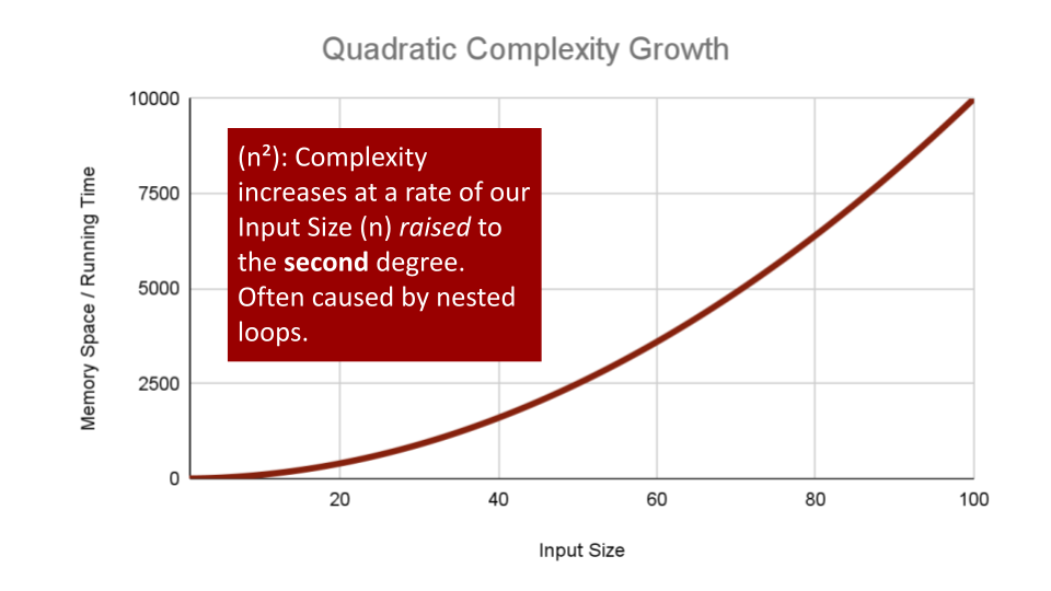
Quadratic Complexity describes an algorithm with complexity growing at a rate of input size n multiplied by n. This is often seen in algorithms that have nested loops which perform iterative or recursive logic on all values of n and immediately iterate or recurse again for each value of n.

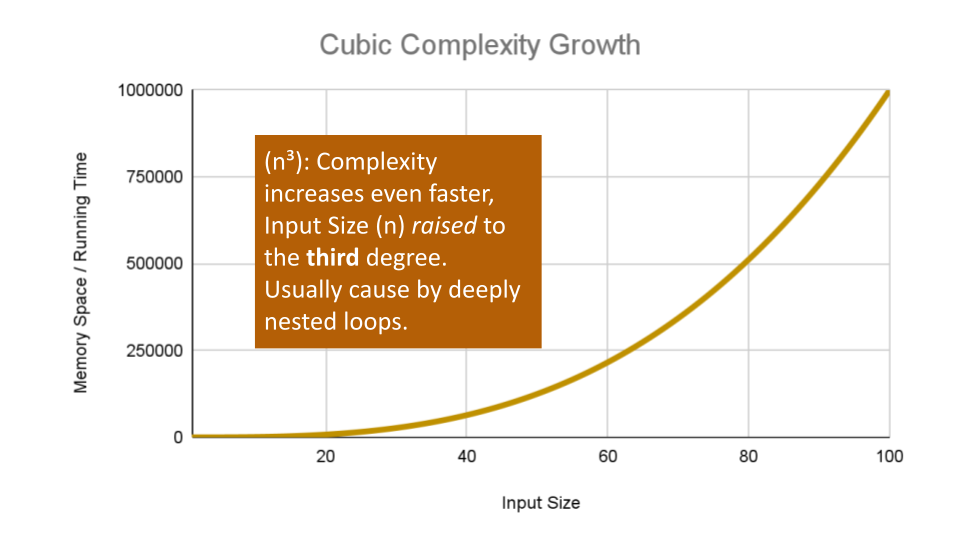
Cubic Complexity is typically just a higher degree of what makes the quadratic complexity grow at such a high rate. We can illustrate this by nesting more loops within our algorithm.

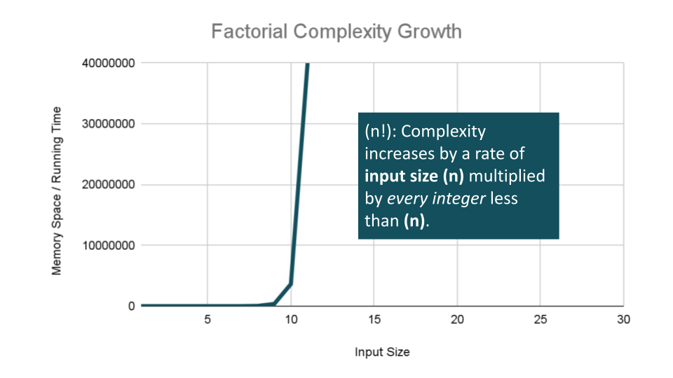
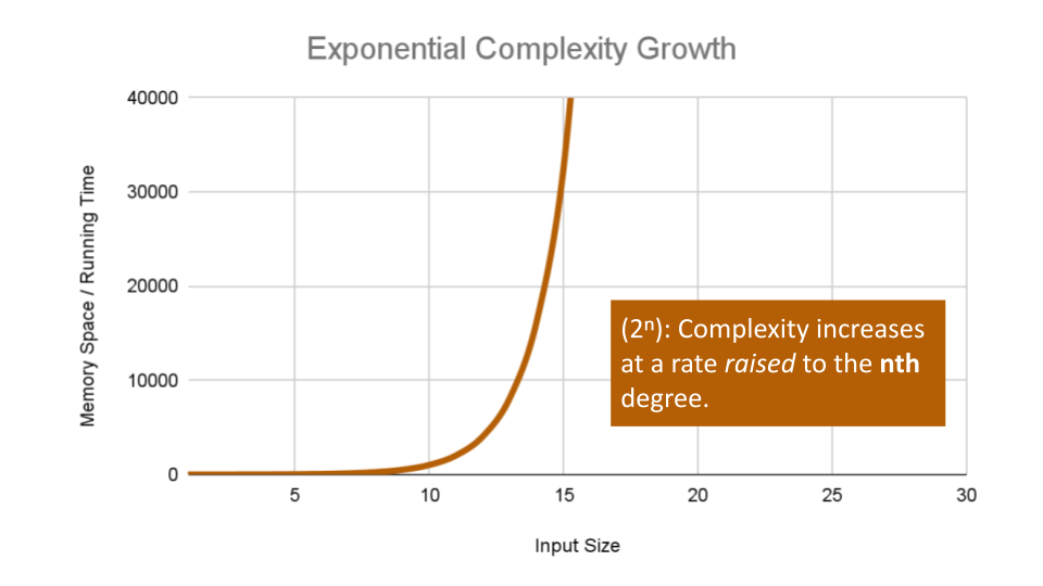
Exponential Complexity represents very rapidly growing complexity, such that whatever our input size n, we are performing the sam number of iterative or recursive loops as n.

Factorial Complexity means that the our space and time requirements grow extremely fast, relative to our input size. At this rate we are performing an extreme amount of calculations for every value within our input of size n.

<—BACK